
In any business operation, it is important to ensure consistency in products as well as repeatable results. Managers and workers alike have to be aware of the processes and methods on how to produce consistent outcomes at all costs. However, we cannot deny that producing exactly identical products or results is almost impossible as variance tends to exist. Variation is not necessarily a bad thing as long as it is within the standard of the critical to qualities (CTQs) specification limits.
Process variation is the occurrence when a system deviates from its fixed pattern and produces a result which differs from the usual ones. This is a major key as it concerns the consistencies of the transactional as well as the manufacturing of the business systems. Variation should be evaluated as it portrays the reliability of the business for the customers and stakeholders. Variation may also cost money hence it is crucial to keep variation at bay to prevent too much cost spent on variation. It is crucial to be able to distinguish the types of variance that occur in your business process since it will give the lead on what course of action to take. Mistakes in coming up with an effective reaction plan towards the variance may worsen the processes of the business.
There are two types of process variation which will be further elaborated in this article. The variations are known as common cause variation and special cause variation.
Common Cause Variation Definition
Common cause variation refers to the natural and measurable anomalies that occur in the system or business processes. It naturally exists within the system. While it is true that variance may bring a negative impact to business operations, we cannot escape from this aspect. It is inherent and will always be. In most cases, the common cause variant is constant, regular, and could be predicted within the business operations. The other term used to describe this variation is Natural Problems, Noise, or Random Cause. Common cause variance could be presented and analysed using histogram.
What is Common Cause Variation
There are several distinguishable characteristics of common cause variation. Firstly, the variation pattern is predictable. Common cause variation occurring is also an active event in the operations. it is controlled and is not significantly different from the usual phenomenon.
There are many factors and reasons for common cause variation and it is quite difficult to pinpoint and eliminate them. Some common cause variations are accepted within the business process and operations as long as they are within a tolerable level. Eradicating them is an arduous effort unless a drastic measure is implemented towards the operation.
Common Cause Variation Examples
There is a wide range of examples for common cause variation. Let’s take driving as an example. Usually, a driver is well aware of their destinations and the conditions of the path to reach the destination. Since they have been regularly using the same road, any defects or problems such as bumps, conditions of the road, and usual traffic are normal. They may not be able to precisely arrive at the destination at the same duration every time due to these common causes. However, the duration to arrive at the destination may not be largely differing day to day.
In terms of project-related variations, some of the examples include technical issues, human errors, downtime, high trafficking, poor computer response times, mistakes in standard procedures, and many more. Some other examples of common causes include poor design of products, outdated systems, and poor maintenance. Inconducive working conditions may also result in to common cause variants which could comprise of ventilation, temperature, humidity, noise, lighting, dirt, and so forth. Errors such as quality control and measurement could also be counted as common cause variation.
Special Cause Variation Definition
On the other hand, special cause variation refers to the unforeseen anomalies or variance that occurs within business operations. This variation, as the name suggests, is special in terms of being rare, having non-quantifiable patterns, and may not have been observed before. It is also known as Assignable Cause. Other opinions also mentioned that special cause variation is not only variance that happens for the first time, a previously overlooked or ignored problem could also be considered a special cause variation.
What is Special Cause Variation
Special cause variation is irregular occurrences and usually happens due to changes that were brought about in the business operations. It is not your mundane defects and may be very unpredictable. Most of the time, special cause variation happens following the flaws within the business processes or mechanism. While it may sound serious and taxing, there are ways to fix this which is by modifying the affected procedures or materials.
One of the characteristics of special cause variation is that it is uncontrolled and hardly predictable. The outcome of special causes variation is significantly different from the usual phenomenon. Since the issues are not predictable, it is usually problematic and may not even be recorded in the historical experience base.
Special Cause Variation Examples
As mentioned earlier, special cause variations are unexpected variants that occur due to factors that may affect the business system or operations. Let’s have an example of a special cause using the same scenario as previously elaborated for common cause variation example. The mentioned defects were common. Now, imagine if there is an unexpected accident that happens on the same road you usually take. Due to this accident, the time for the driver to arrive at the same destination may take longer than normal. Hence this accident is considered as a special cause variation. It is unexpected and results in a significantly different outcome, in this case, a longer time to arrive at the destination.
The example of special cause variation in the manufacturing sector includes environment, materials, manpower, technology, equipment, and many more. In terms of manpower, imagine a new employee is recruited into the team and still lacking in experience. The coaching and instructions should be adapted to consider that the person needs more training to be able to perform their tasks efficiently. Cases where a new supplier is needed in a short amount of time due to issues faced by the existing supplier are also unforeseen hence considered a special cause variation. Natural hazards that are beyond predictions may also be categorized into special cause variation. Some other examples include irregular traffic or fraud attack. An unexpected computer crash or malfunction in some of the components may also be considered as a special cause variation.
Common Cause and Special Cause Variation Detection
Control chart
One of the ways to keep track of common cause and special cause variation is by implementing control charts. When using control charts, the important aspect to be considered is firstly, establishing the average point of measurement. Next, establish the control limits. Usually, there are three standard deviations which are marked above and below the average point earlier. The last step is by determining which points exceed the upper and lower control limits established earlier. The points beyond the limits are special cause variation.
Before we get into the control chart of common cause and special cause variation, let’s have a look at the eight control chart rules first. If a process is stable, the points displayed in the chart will be near the average point and will not exceed the control limits.
| No | Rule Name | Pattern |
| 1 | Beyond Limits | One or more points exceed control limits |
| 2 | Zone A | 2 out of 3 continuous points in Zone A or beyond |
| 3 | Zone B | 4 out of 5 continuous points in Zone B or beyond |
| 4 | Zone C | 7 or more continuous points in Zone C or beyond |
| 5 | Trend | 7 consecutive points inclining upwards or downwards |
| 6 | Mixture | 8 continuous point with no points in Zone C |
| 7 | Stratification | 15 continuous points in Zone C |
| 8 | Over-control | 14 continuous points alternating up and down |
However, it should be noted that not all rules are applicable to all types of control charts. That aside, it is quite tough to identify the causes of the patterns since special cause variation may be related to the specific type of processes. The table presented is the general rule that could be applied in most cases but is also subject to changes or differences. Studying the chart should be accompanied by knowledge and experiences in order to pinpoint the reasons for the patterns or variations.
A process is considered stable if special cause variation is not present, even if a common cause exists. A stable operation is important before it could be assessed or being improved. We could look at the stability or instability of the processes as displayed in control charts or run charts.
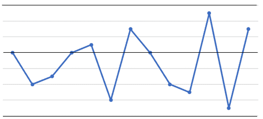
The points displayed in the chart above are randomly distributed and do not defy any of the eight rules listed earlier. This indicates that the process is stable.
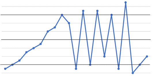
The chart presented above is an example of an unstable process. This is because some of the rules for control chart tests mentioned earlier are violated.
Simply, if the points are randomly distributed and are within the limit, they may be considered as the common cause variation. However, if there is a drastic irregularity or points exceeding the limit, you may want to analyse more into it to determine if it is a special cause variation.
Histogram
Histogram is a type of bar graph that could be used to present the distribution of occurrences of data. It is easily understandable and analysed. A histogram provides information on the history of the processes done as well as forecasting the future performance of the operations. To ensure the reliability of the data presented in the histogram, it is essential for the process to be stable. As mentioned earlier, although affected by common cause variation, the processes are still considered stable, hence histogram may be used on this occasion, especially if the processes undergo regular measurement and assessment.
The data is considered to be normally distributed if it portrays a “bell” shape in the histogram. The data are grouped around the central value and this cluster is known as variation. There are several other examples of more complicated patterns, such as having several peaks in the histogram or a shortened histogram. Whenever these examples of complex structures appear in the histogram, it is fundamental to look into the data and operations more deeply.
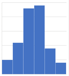
The above bar graph is an example of the histogram with a “bell” shape.
However, it should be noted that just because the histogram displays a “bell” shaped distribution, that does not mean the process is only experiencing common cause variation. A deeper analysis should be done to investigate if there were other underlying factors or causes that lead towards the pattern of the distribution displayed in the histogram.
Countering common cause and special cause variation
Once the causes of the variation have been pinpointed, here comes the attempt to combat and resolve it. Different measures are implemented to counter different types of variation, i.e. common cause variation and special cause variation. Common cause variation is quite tough to be completely eliminated. Drastic or long-term process modification could be used to counter common cause variation. A new method should be introduced and constantly conducted to achieve the long-term goal of eliminating the common cause variation. Some other effects may happen to the operations but as time passes, the cause may be gradually solved. As for special cause variation, it could be countered using contingency plans. Usually, additional processes are implemented into the usual operation in order to counter the special cause variation.